Cut Gems

Below is one of my first data visualizations for my quantitative chemistry class. It uses the famous “diamonds” data set.
The full code required to replicate this visualization can be found at the bottom of this page.

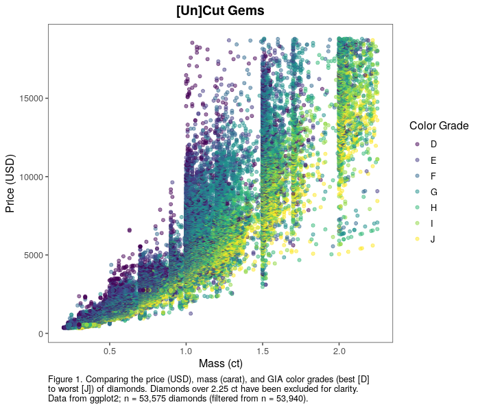
From the figure, it can be concluded that higher color grade diamonds sell for higher prices than those of a lower grade with the same mass. However, a unique relationship can be seen between the higher-carat diamonds (those over 2.0 ct) and price without the additional factor of color grade; even the low color grade diamonds over 2.0 ct are being sold for considerably high prices. There also appear to be fewer high color grade diamonds over 1.75 ct.
It should be noted that although the color grades are being categorized as “best” to “worst”, the full GIA color grade scale ranges from D to Z; diamonds graded as J are still considered to be near-colorless. If the dataset had included the lower color grades, it would be interesting to see the ranges of price for them as well. Additional factors to explore would be the relationships between the variables presented in the figure and those included in the dataset but not depicted above: cut, clarity, and various size measurements.

## Loading necessary libraries.
library(tidyverse)
library(ggplot2)
library(ggthemes)

## Filtering major outliers to make a cleaner plot.
diamonds_mod <- diamonds %>%
filter(carat <= 2.25)

## Creating the plot.
ggplot(data = diamonds_mod,
    mapping = aes(x = carat,
                    y = price,
                    color = color))+
geom_point(alpha = 0.5)+
theme_few()+
labs(x = "Mass (ct)",
    y = "Price (USD)",
    color = "Color Grade",
    title = "[Un]Cut Gems",
    caption = "Figure 1. Comparing the price (USD), mass (carat), and GIA color grades (best [D]\nto worst [J]) of diamonds. Diamonds over 2.25 ct have been excluded for clarity.\nData from ggplot2; n = 53,575 diamonds (filtered from n = 53,940).")+
theme(plot.title = element_text(hjust = 0.5, face = "bold"),
        plot.caption = element_text(hjust = 0))

## Bonus plot / playing around
# ggplot(diamonds_mod, aes(
# x = carat,
# y = price,
# color = color)
# )+
# geom_point(alpha = 0.25)+
# facet_wrap("cut")